Very very basic ODE and Phase Diagrams
Linear ODEs & Phase Diagrams
Solving Linear First-Order ODEs
How to solve Linear ODE
Given: \(\frac{dy}{dt} - ay = -b\)
Multiply both sides by $e^{-at}$:
\[e^{-at}\frac{dy}{dt} - a \cdot e^{-at} y = -b \cdot e^{-at}\]The boxed expression looks like the derivative of $e^{-at} \cdot y$, since:
\[\frac{d(e^{-at} \cdot y)}{dt} = e^{-at}\frac{dy}{dt} + y \cdot e^{-at}(-a) = e^{-at}\frac{dy}{dt} - aye^{-at}\]Thus: \(\frac{d(e^{-at} \cdot y)}{dt} = -b \cdot e^{-at}\)
\[d(e^{-at} \cdot y) = -b\cdot e^{-at}\, dt\]Integrating both sides: \(\int d(e^{-at} \cdot y) = \int -b\cdot e^{-at}\, dt\)
\[e^{-at} \cdot y = \frac{be^{-at}}{a} + C\] \[y = \frac{b}{a} + \frac{C}{e^{-at}} = \frac{b}{a} + Ce^{at}\] \[\boxed{y = \frac{b}{a} + Ce^{at}}\]The Integrating Factor — Intuition
In the previous question, we multiplied both sides by $e^{-at}$. That particular term is called the integrating factor.
What’s the use?
As we saw in the example, when we multiplied both sides by $e^{-at}$ (integrating factor), we found an anti-derivative. We could guess what the anti-derivative would look like.
Generally, the linear ODE looks like: \(\frac{dy}{dt} + P(x)\cdot y = Q(x)\)
We find the integrating factor by: \(\text{I.F.} = e^{\int P(x)\, dx}\)
Now, multiplying both sides by I.F.: \(\text{I.F.}\cdot\frac{dy}{dx} + P(x)\cdot y \times \text{I.F.} = Q(x)\cdot \text{I.F.}\)
\[\Rightarrow \frac{d(\text{I.F.}\cdot y)}{dx} = Q(x)\cdot \text{I.F.}\]Now, proceed with integration.
Example: \(\frac{dy}{dx} + \underbrace{3x^2}_{P(x)}y = \underbrace{6x^2}_{Q(x)}\)
Solution to Example
\(y = 2 + Ce^{-x^3}\)
Part 2: Phase Diagrams
Introduction
\[\dot{y_1} = \frac{dy_1}{dt} = 0.06y_1(t) - y_2(t) + 1.4\] \[\dot{y_2} = \frac{dy_2}{dt} = -0.004y_1(t) + 0.04\]Reading or drawing a phase diagram is really no easy [sic — “not”] Rocket Science. Suppose we’re given 2 simple ODEs:
Step 1: First we need to equate $\dot{y_1}=0$, $\dot{y_2}=0$, to get two lines which show the relationship between $y_1(t)$ and $y_2(t)$.
- $\dot{y_1}=0 \Rightarrow y_2(t) = 0.06y_1(t) + 1.4$
- $\dot{y_2}=0 \Rightarrow y_1(t) = 10$
Drawing the Axes
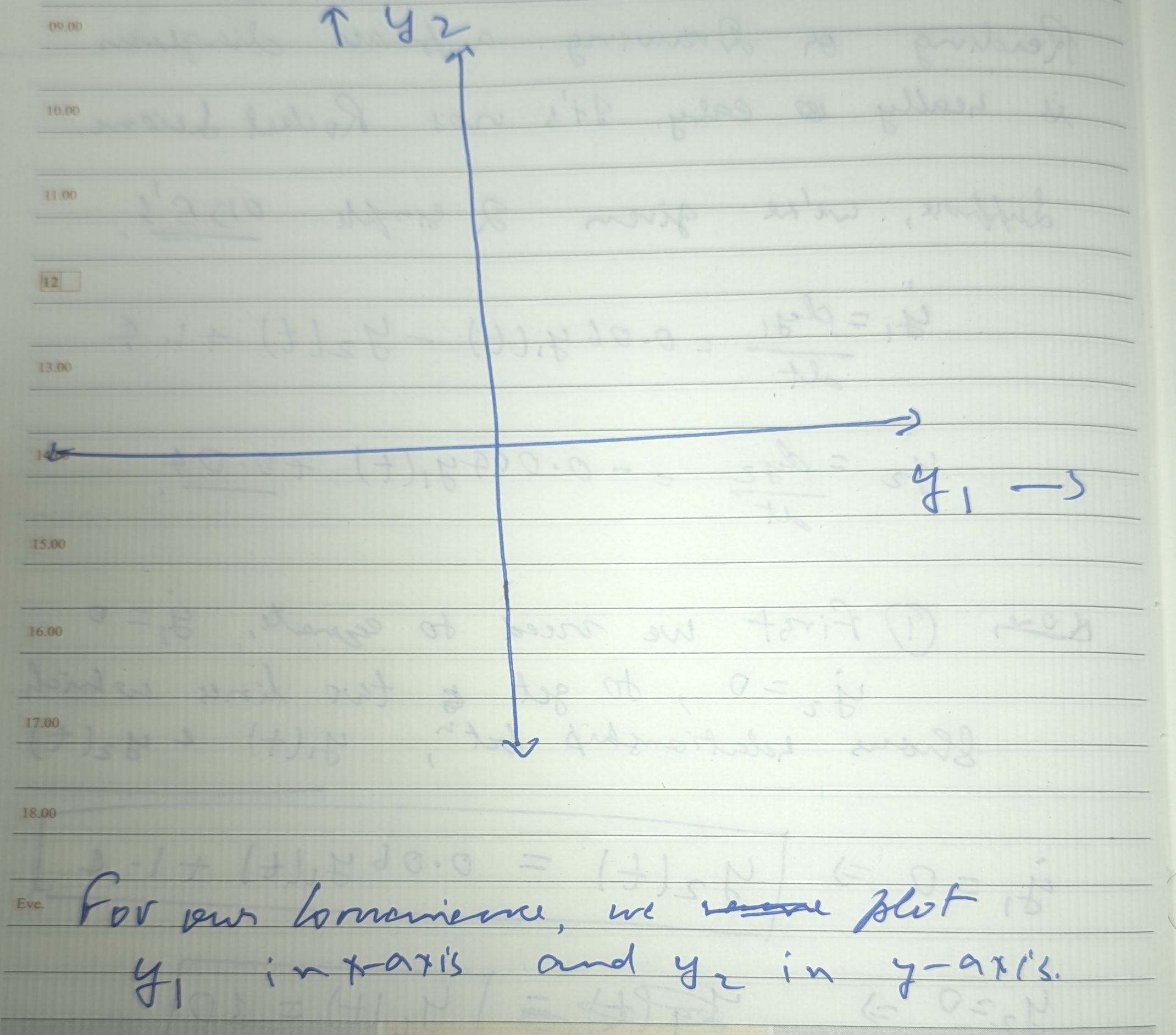
Now, let’s draw the graph first. For our convenience, we plot $y_1$ in the x-axis and $y_2$ in the y-axis.
Plotting the Nullclines
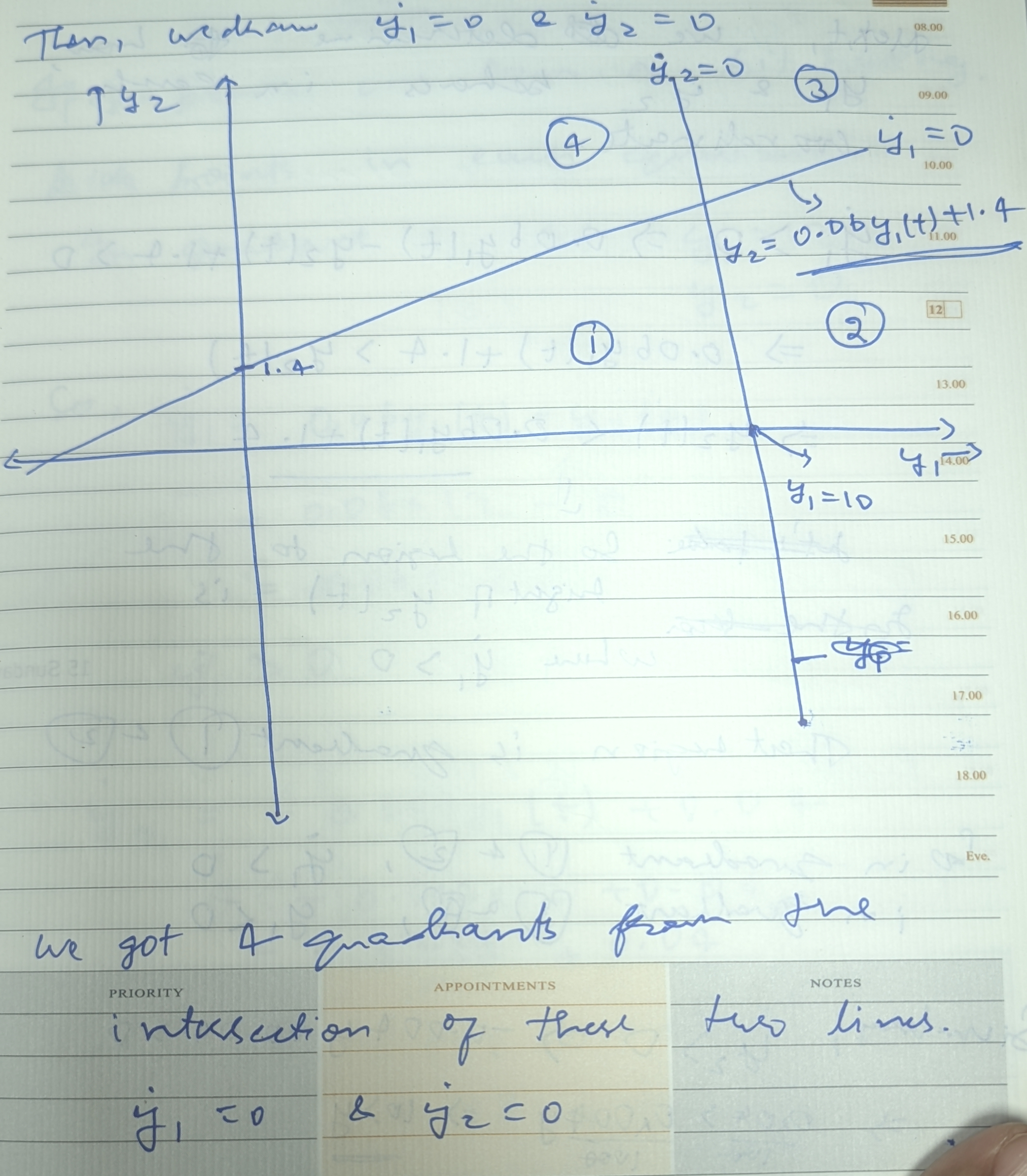
Then, we draw $\dot{y_1}=0$ and $\dot{y_2}=0$.
- Line $\dot{y_2}=0$: $y_2 = 0.06y_1(t) + 1.4$ (upward sloping line, intercept 1.4)
- Line $\dot{y_1}=0$: $y_1 = 10$ (vertical line)
We got 4 quadrants from the intersection of these two lines.
Determining Behavior in Each Region
Next, we determine how $y_1$ and $y_2$ behave in each coordinate.
\(y_1 > 0 \Rightarrow 0.06y_1(t) - y_2(t) + 1.4 > 0\) \(\Rightarrow 0.06y_1(t) + 1.4 > y_2(t)\) \(\Rightarrow y_2(t) < 0.06y_1(t) + 1.4\)
So the region to the right of $y_2(t)$ is where $\dot{y_1} > 0$.
That region is Quadrants ① and ②.
- In Quadrants ① and ②: $\dot{y_1} > 0$
- In Quadrants ③ and ④: $\dot{y_1} < 0$
Similarly, $\dot{y_2} > 0 \Rightarrow -0.004y + 0.04 > 0$
\[\Rightarrow \frac{0.04}{100} > \frac{0.004y}{1000} \Rightarrow 10 > y\]- In Quadrants ① and ④: $\dot{y_2} > 0$
Alternative Method
If the previous one seems a bit hectic, plug points in each quadrant.
In Quadrant 1, let $y_1 = 12$, $y_2 = 0$:
\[\dot{y_1} = 0.06y_1(t) - y_2(t) = 0.06(12) - 0 = 0.72 > 0\] \[\dot{y_1} > 0\] \[\dot{y_2} = -0.004y_1(t) + 0.04 = -0.004(12) + 0.04 = -\frac{12\times4}{1000} + 0.04 = -0.048+0.04 = -0.008\] \[\dot{y_2} < 0\]Repeating for All Quadrants
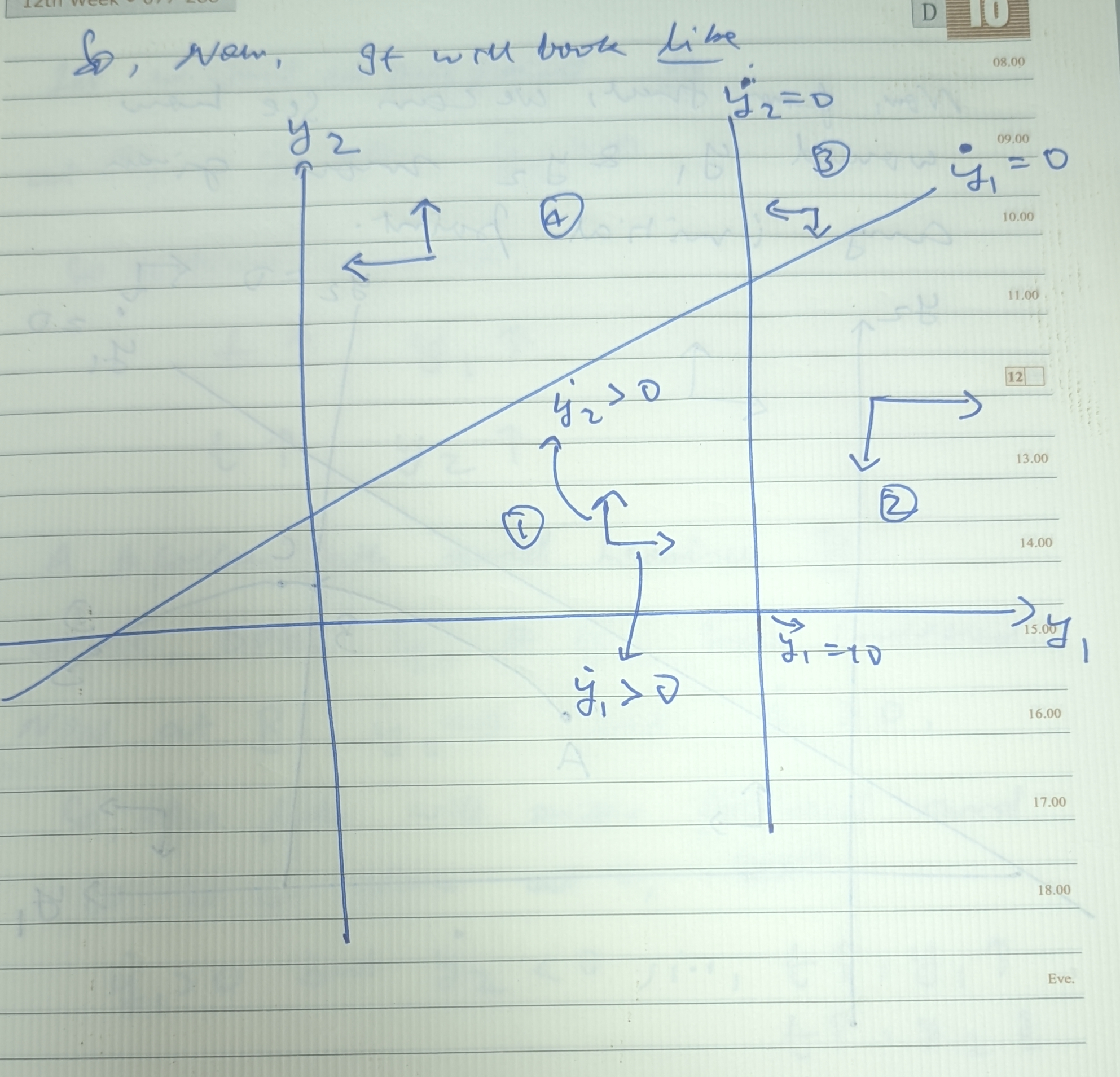
Repeat the same for all quadrants. Eventually you’ll come to this:
- Quadrant 1: $\dot{y_1} > 0,\ \dot{y_2} > 0$
- Quadrant 2: $\dot{y_1} > 0,\ \dot{y_2} < 0$
- Quadrant 3: $\dot{y_1} < 0,\ \dot{y_2} < 0$
- Quadrant 4: $\dot{y_1} < 0,\ \dot{y_2} > 0$
Direction Arrows
Now, let’s see how would $y_1$ & $y_2$ move given any initial point.
Arrows are drawn in each quadrant showing the direction of motion implied by the signs of $\dot{y_1}, \dot{y_2}$ (e.g., Quadrant ① → up-right, Quadrant ③ → down-left, etc.), consistent with the sign table above.
Tracing a Trajectory
Now, from that, we can see how would $y_1$ & $y_2$ move given any initial point.
Let us start at point A:
At $A$: $\dot{y_1} > 0,\ \dot{y_2} > 0$
So as time increases: \(t\uparrow \Rightarrow y_1\uparrow\) \(t\uparrow \Rightarrow y_2\uparrow\)
- Path from A follows and reaches B.
- At B, both $y_1$ and $y_2$ have increased. At B: $\dot{y_2}=0$ but $\dot{y_1}>0$.
- So the path moves forward and goes to C.
- At C: $\dot{y_1}>0$ but $\dot{y_2}<0$, i.e., $t\uparrow, y_1\uparrow$ and $t\uparrow, y_2\downarrow$.
- So now, direction of the path changes — it moves towards D.
This traces out a curved trajectory (A → B → C → D) that rises, peaks near the $\dot{y_2}=0$ nullcline, and then declines — consistent with the vector-field arrows in each quadrant of the phase diagram.
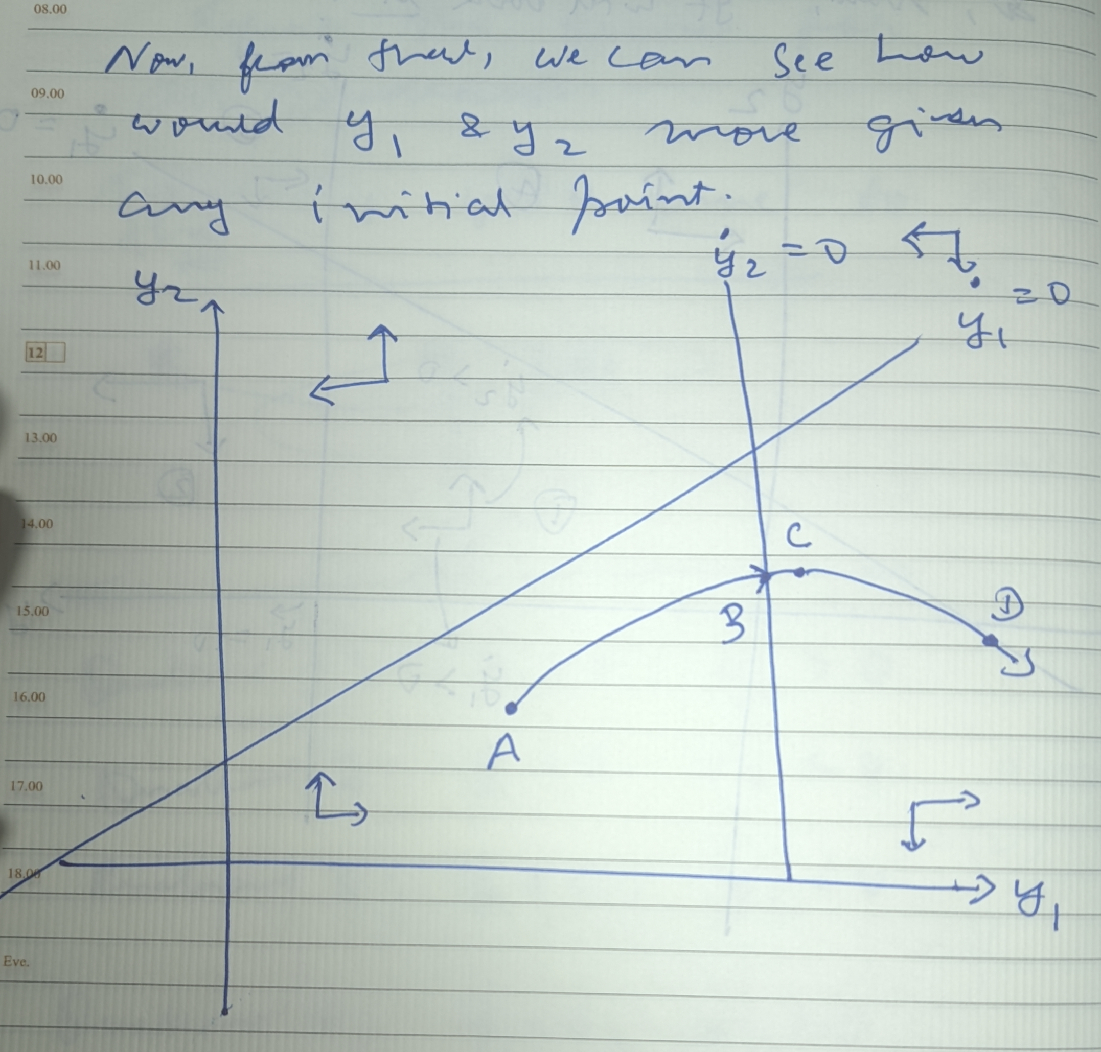
Note: The curved arrows and the A→B→C→D path above are only meant to illustrate how a phase diagram is read — they are not a literal plot of the actual solution $(y_1(t), y_2(t))$.
In reality, how fast $y_1$ and $y_2$ move (and how curved their joint path looks) depends on the actual coefficients in each equation — some variables can change very quickly while others barely move, so the true trajectory could be almost flat, almost vertical, or heavily curved depending on the relative speeds of $\dot{y}_1$ and $\dot{y}_2$.
The path also depends entirely on where you start (the initial point) — a different starting point can land in a different quadrant, follow a completely different route toward (or away from) the nullclines, and even approach the equilibrium from the opposite direction.
So: read this diagram for the logic of phase analysis — which quadrant pushes $y_1$ and $y_2$ which way, and how the direction of motion changes as you cross a nullcline — not as a precise picture of the system’s real dynamics.